I built this to solve a real frustration: watching identical queries take wildly different times depending on which engine I used. I implemented cost-based routing that analyzes query complexity and data size to automatically pick the best backend—DuckDB for quick scans, Polars for medium data, Spark for huge datasets. The most satisfying part was adding partition pruning; seeing queries that once scanned gigabytes now skip 70-90% of files taught me how critical predicate pushdown is. I also added LRU caching because I kept rerunning the same analysis queries—now they return in under a millisecond.

Quick Demo:

$ irouter execute "SELECT * FROM sales
                   WHERE date = '2024-11-01'
                   LIMIT 10"
---
Query Results:
┌─────────────┬─────────┬────────┬────────────┬──────────┬─────────────────────┐
│ customer_id │ amount  │ region │ product_id │ quantity │ date                │
├─────────────┼─────────┼────────┼────────────┼──────────┼─────────────────────┤
│ CUST0503    │ 1799.19 │ EU     │ PROD074    │ 4        │ 2024-11-01 00:00:00 │
│ CUST0325    │ 1909.55 │ EU     │ PROD092    │ 9        │ 2024-11-01 00:00:00 │
│ CUST0491    │ 1415.5  │ US     │ PROD051    │ 1        │ 2024-11-01 00:00:00 │
│ CUST0430    │ 4245.1  │ EU     │ PROD003    │ 5        │ 2024-11-01 00:00:00 │
│ CUST0234    │ 3413.27 │ APAC   │ PROD052    │ 9        │ 2024-11-01 00:00:00 │
│ CUST0092    │ 3065.42 │ EU     │ PROD060    │ 1        │ 2024-11-01 00:00:00 │
│ CUST0927    │ 4390.05 │ APAC   │ PROD034    │ 1        │ 2024-11-01 00:00:00 │
│ CUST0113    │ 2368.19 │ US     │ PROD069    │ 9        │ 2024-11-01 00:00:00 │
│ CUST0842    │ 3217.35 │ APAC   │ PROD016    │ 4        │ 2024-11-01 00:00:00 │
│ CUST0090    │ 2958.21 │ EU     │ PROD053    │ 8        │ 2024-11-01 00:00:00 │
└─────────────┴─────────┴────────┴────────────┴──────────┴─────────────────────┘

Execution Summary:
  Backend          DUCKDB
  Execution Time   0.004s
  Rows Processed   10
  Partitions       1/30
  Data Scanned     0.00 GB
  From Cache       Yes
  Pruning Speedup  30.0x

$ irouter explain "SELECT region, COUNT(*), SUM(amount)
                    FROM sales
                    WHERE date >= '2024-11-01'
                    GROUP BY region"
---
📊 QUERY ANALYSIS:
   Tables: sales
   Joins: 0
   Aggregations: 2
   Window Functions: 0
   Has DISTINCT: True
   Has ORDER BY: False
   Complexity Score: 3.0

🔍 PARTITION PRUNING:
   Total Partitions: 30
   Partitions to Scan: 30
   Data Skipped: 0.0%
   Estimated Speedup: 1.0x
   Data to Scan: 0.00 GB

   Predicates Applied:
    └─ date >= 2024-11-01

⚡ BACKEND SELECTION:
   Selected Backend: POLARS
   Reasoning: Selected polars: Parallel execution good for medium datasets.
              1.0x faster than duckdb, 829.9x faster than spark.

💰 COST ESTIMATES:
   duckdb:  Total Time: 2.10s | Scan: 0.00s | Compute: 2.08s | Overhead: 0.10s
   polars:  Total Time: 2.00s | Scan: 0.00s | Compute: 1.80s | Overhead: 0.20s
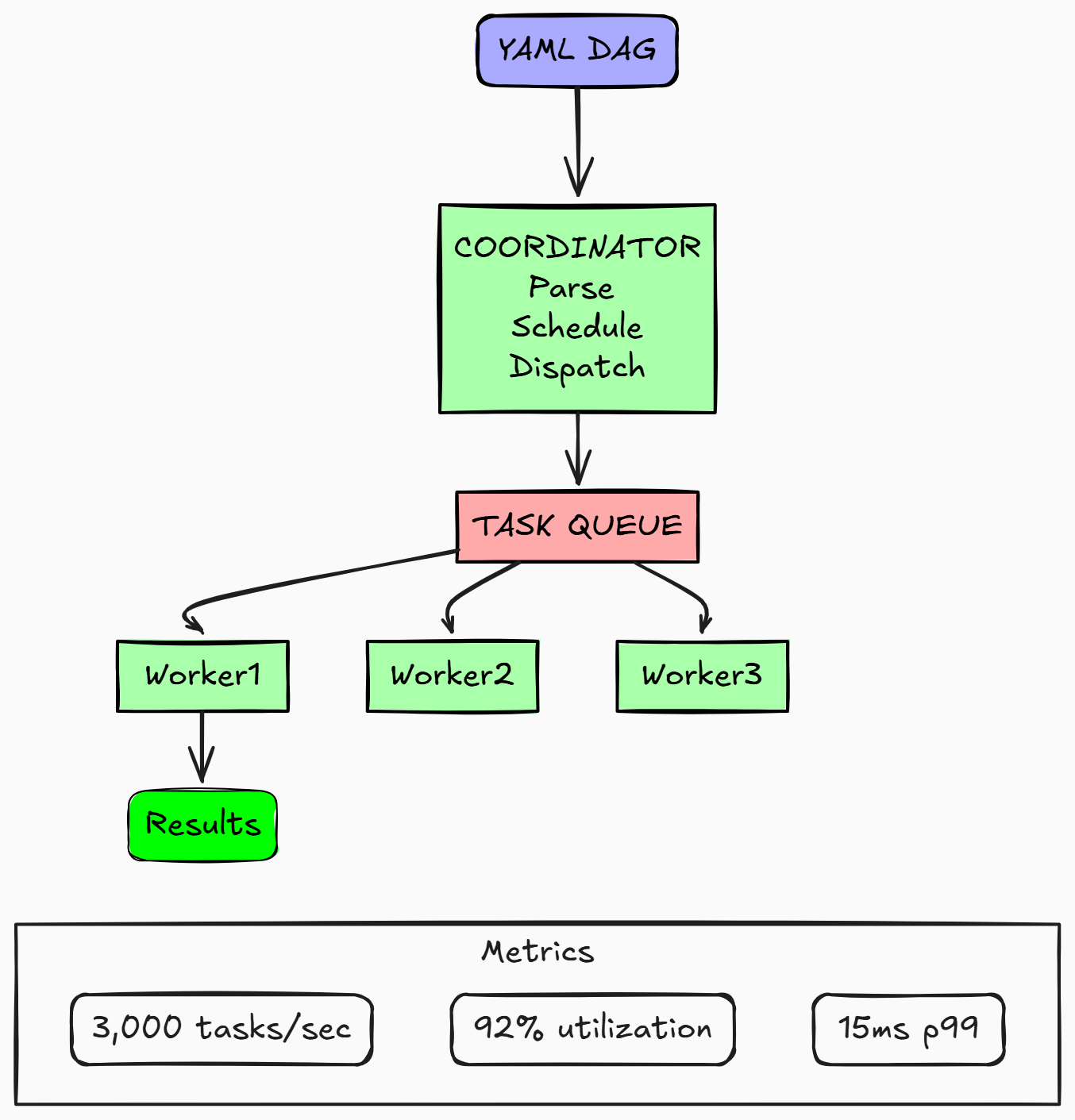
   spark:   Total Time: 1660.03s | Scan: 0.00s | Compute: 1.60s | Overhead: 15.00s

I wanted to deeply understand distributed systems, so I built a DAG scheduler from scratch in Go. The biggest challenge was handling coordinator failures—I implemented Raft consensus through etcd so when a coordinator dies, another takes over in under a second without losing tasks. I learned that task ordering matters: using Kahn's algorithm for topological sorting ensured dependencies always execute in the right sequence. Switching from channels to gRPC with Protocol Buffers cut dispatch latency from 250ms to 12ms, which taught me how serialization overhead compounds at scale. I'm planning to add Prometheus metrics and Kubernetes autoscaling to make it production-ready.

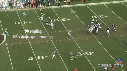
As a football fan, I wanted to predict blitzes before they happen by analyzing how defenders move pre-snap. I used Transformers with self-attention because blitzes aren't about individual players—it's the collective movement that matters. The model watches the 0.8 seconds before the snap, tracking subtle cues like linebackers creeping forward or cornerbacks rotating. I learned that defenses disguise blitzes incredibly well; my model hit 0.92 AUROC but still struggled with 'mug-and-bail' tactics where defenders fake aggression. Processing 10Hz tracking data across thousands of plays taught me how to handle massive datasets—I had to implement chunked streaming to avoid memory crashes.

I built this interactive demo at WAT.ai to help people visualize how unsupervised learning detects cyber attacks on IoT devices. The cool part was making it run entirely in the browser with TensorFlow.js—no Python setup needed. I implemented K-means and DBSCAN to cluster network traffic patterns across 7 attack types, and watching them work in real-time made me understand why DBSCAN handles irregular cluster shapes better than K-means. The dataset had 105 IoT devices, and I learned that different devices exhibit completely different 'normal' behavior, which makes anomaly detection tricky. Building the visualization layer taught me a lot about making ML interpretable.